Calculating full-year energy savings with only 6 months of data

A Python tutorial using LightGBM

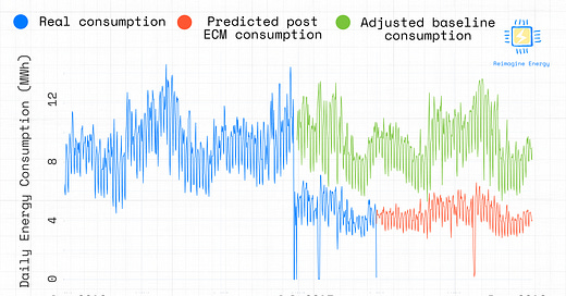
Just another day in the life of a building energy manager: you've implemented an energy conservation measure (ECM), collected some data, and now you need to report the annual savings... but you only have 6 months of data.

This happened to me recently. I wanted to analyze how solar panel savings change when combined with other energy conservation measures. So I set out to combine a full year of on-site panels’ production with the building’s consumption before and after implementing an ECM. The issue was that I only had 6 months of post-implementation data and I needed a full year to make accurate comparisons.

So I asked myself: Could we predict the next 6 months of consumption based on the historical data from the building and on the patterns we see in the first 6 months of post-ECM data?

In this tutorial, I'll show you how to use LightGBM to extrapolate your partial-year energy savings into a full-year estimate. We'll build a model that learns from your building's energy patterns and predicts future consumption.

Getting Started

First, we need to import the necessary libraries:

import pandas as pd
import lightgbm
import plotly.graph_objects as go

Loading electricity consumption data

We’re using data from the Building Data Genome Project 2. For details on this dataset and how to handle it, have a look at our previous tutorial:

# Read electricity consumption file

meters_df = pd.read_csv('data/electricity_cleaned.csv')

# Set the timestamp column as index of the dataframe

meters_df.set_index('timestamp', inplace=True)
meters_df.index = pd.to_datetime(meters_df.index)

# Create a new dataframe with only the data for the selected building

building_df = meters_df['Rat_education_Alfonso']
building_df = building_df.rename('consumption')

Loading and preprocessing weather data

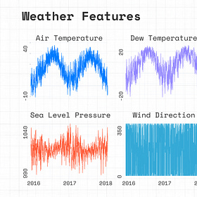
We’ll need weather data for 2016, 2017, and 2018. I downloaded this data from the National Solar Radiation Database, but any historical weather data source will do.

# Process and combine 3 years of weather data files (2016-2018)
# Each file needs special handling since first row contains metadata:
# 1. Drop first row which contains metadata
# 2. Use the new first row as column headers
# 3. Reset index to avoid duplicate indices when concatenating

# The function below handles this preprocessing for each weather file
def process_weather_file(filepath):
    df = pd.read_csv(filepath)
    df = df.iloc[1:].copy()  # Drop first row and make copy
    df.columns = df.iloc[0]  # Set column names from first row
    return df.iloc[1:].reset_index(drop=True)  # Drop the header row and reset index

# Process all weather files
weather_files = [
    'data/washington_dc_weather_2016.csv',
    'data/washington_dc_weather_2017.csv', 
    'data/washington_dc_weather_2018.csv'
]
weather_dfs = [process_weather_file(f) for f in weather_files]

# Concatenate all dataframes
weather_df = pd.concat(weather_dfs)

# Create datetime index
weather_df['datetime'] = pd.to_datetime(weather_df[['Year', 'Month', 'Day', 'Hour', 'Minute']])
weather_df.set_index('datetime', inplace=True)

# convert values to float
weather_df[['Temperature', 'Wind Speed', 'Wind Direction', 'Pressure', 'Dew Point']] = \
    weather_df[['Temperature', 'Wind Speed', 'Wind Direction', 'Pressure', 'Dew Point']].astype(float)

# select only relevant columns
weather_df = weather_df[['Temperature', 'Wind Speed', 'Wind Direction', 'Pressure', 'Dew Point']]

# resample to hourly
weather_df = weather_df.resample('H').mean()
weather_df.head()

Output

Merging consumption and weather data

Let’s merge the consumption data with the weather data and add features needed for the analysis.

We know from the previous tutorial that the energy conservation measure was implemented on 2017-06-28, let’s add a boolean feature marking the pre- and post-installation periods.

# merge the dataframes keeping all rows from weather_df by using right merge
df = building_df.to_frame().merge(weather_df, left_index=True, right_index=True, how='right')

# Add time-based features
df['hour'] = df.index.hour
df['dayofweek'] = df.index.dayofweek
df['week'] = df.index.isocalendar().week.astype('int')

# add a new column "energy_conservation_measure" which is 1 after the ECM implementation date
df['energy_conservation_measure'] = 0
df.loc[df.index >= pd.to_datetime('2017-06-28'), 'energy_conservation_measure'] = 1

df.head()

Output

In our previous tutorial on counterfactual energy modeling, we had already built a model to estimate the adjusted baseline consumption after the ECM implementation as if the ECM had not been implemented. You can check it out here:

The post-ECM installation data available for this building spans only half a year (from mid 2017 until the end of the year). Our goal is then to estimate what the consumption will be for the year 2018, if it follows the same trend as after the ECM implementation. We’ll also need to calculate an adjusted baseline consumption for the year 2018 to estimate the savings. Let’s define the datasets we need for our analysis.

Defining analysis periods

We need to define key dates and periods for our analysis:

• Pre ECM Period: Before ECM implementation (before June 21, 2017)

• Installation Period: June 21–28, 2017

• Initial Reporting Period: Post-installation until the end of 2017

• Full Reporting Period: All of 2018

# Define key dates for analysis

installation_start = pd.to_datetime('2017-06-21')
installation_end = pd.to_datetime('2017-06-28')
last_consumption_date = pd.to_datetime('2017-12-31')

training_data_pre_ecm = df[df.index <= installation_start]
training_data_full_period = df[df.index <= last_consumption_date]
prediction_data_post_ecm = df[df.index >= installation_end]
prediction_data_2018 = df[df.index > last_consumption_date]

Baseline model function

We’ll use LightGBM to build our baseline model.

# define function to build baseline model

def build_baseline_model(data, target_variable, features, seed=None):

    data = data.dropna(subset=[target_variable])
    X = data[features]

    y = data[target_variable]
    dataset = lightgbm.Dataset(X, y)

    objective = "l2"
    lgbm_params = dict(
        boosting_type="gbdt",
        n_jobs=1,
        objective=objective,
        seed=seed or 42,
        verbosity=0,
    )
    cv = lightgbm.cv(
        params=lgbm_params,
        train_set=dataset,
        stratified=False,
        num_boost_round=200,
        nfold=5,
        callbacks=[lightgbm.early_stopping(5)],
    )

    # Full model (use best num-rounds from cross-validation)

    model = lightgbm.train(
        params=lgbm_params,
        train_set=dataset,
        num_boost_round=len(cv[f"valid {objective}-mean"]),
    )

    # Predict

    y_pred = pd.Series(model.predict(X), index=X.index)

    return {
        "data": data,
        "features": features,
        "target": target_variable,
        "seed": seed,
        "params": lgbm_params,
        "estimator": model,
        "cv": cv,
        "preds": y_pred,
    }

Predicting consumption for 2018

Now, we’ll predict the building’s consumption for the year 2018.

# Define features and train model

features = df.columns.tolist()
features.remove('consumption')

baseline_model = build_baseline_model(
    data=training_data_full_period,
    target_variable='consumption',
    features=features
)

# Make predictions on reporting data
predicted_consumption_post_ecm = pd.Series(
    baseline_model['estimator'].predict(prediction_data_2018[features]), 
    index=prediction_data_2018.index
)

Visualizing the results

Let’s plot the actual consumption and the predicted consumption for 2018.

# plot the actual consumption and the predicted consumption for 2018

fig = go.Figure()

fig.add_trace(go.Scatter(x=training_data_full_period.resample('1D').sum().index, y=training_data_full_period.resample('1D').sum()['consumption'], line=dict(color='#007BFF')))

fig.add_trace(go.Scatter(x=predicted_consumption_post_ecm.resample('1D').sum().index, y=predicted_consumption_post_ecm.resample('1D').sum(), line=dict(color='#ff5733')))

fig.show()

Output

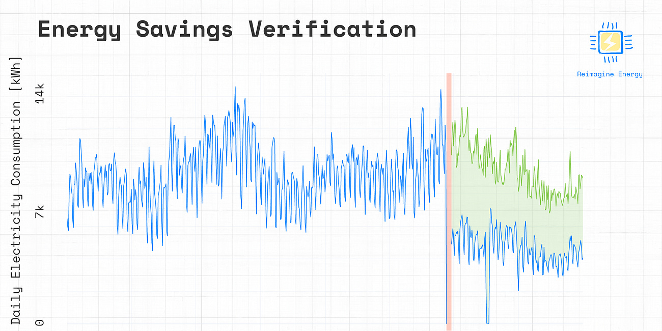
The model seems to perform well, the 2018 predictions align closely with the consumption patterns observed after the ECM implementation in 2017.

Calculating the adjusted baseline consumption

Next, we’ll calculate the adjusted baseline consumption for the full year 2018, representing what consumption would have been without the ECM.

# Estimate adjusted baseline consumption for the post-installation period

adjusted_baseline_model = build_baseline_model(
    data=training_data_pre_ecm,
    target_variable='consumption',
    features=features
)

adjusted_baseline_consumption_post_ecm = pd.Series(
    adjusted_baseline_model['estimator'].predict(prediction_data_post_ecm[features]), 
    index=prediction_data_post_ecm.index
)

Visualizing all results

Let’s plot the actual consumption, adjusted baseline consumption, and predicted consumption for 2018.

# Plot the actual consumption, the adjusted baseline consumption, and the predicted (post-ECM)consumption for 2018
fig = go.Figure()

fig.add_trace(go.Scatter(x=adjusted_baseline_consumption_post_ecm.resample('1D').sum().index, y=adjusted_baseline_consumption_post_ecm.resample('1D').sum(), line=dict(color='#7ac53c')))

fig.add_trace(go.Scatter(x=training_data_full_period.resample('1D').sum().index, y=training_data_full_period.resample('1D').sum()['consumption'], line=dict(color='#007BFF')))

fig.add_trace(go.Scatter(x=predicted_consumption_post_ecm.resample('1D').sum().index, y=predicted_consumption_post_ecm.resample('1D').sum(), line=dict(color='#ff5733')))

fig.show()

Output

Calculating full-year savings

Finally, we’ll calculate the estimated electricity savings for a full year after the ECM implementation.

# Calculate savings for a full year after the ECM implementation

real_consumption_after_ecm = prediction_data_post_ecm['consumption'].sum()

predicted_consumption_one_year_after_ecm = predicted_consumption_post_ecm[predicted_consumption_post_ecm.index < (installation_end + pd.DateOffset(years=1))].sum()

adjusted_baseline_one_year_post_ecm = adjusted_baseline_consumption_post_ecm[adjusted_baseline_consumption_post_ecm.index < (installation_end + pd.DateOffset(years=1))].sum()

full_year_savings = adjusted_baseline_one_year_post_ecm - predicted_consumption_one_year_after_ecm - real_consumption_after_ecm

print(f"Estimated electricity savings for a full year after the ECM implementation: {full_year_savings:.0f} kWh")

Output

Conclusion

With a few lines of code, we’ve extrapolated six months of energy savings to estimate a full year’s worth. This approach is useful when data is limited or when you want to project future savings soon after implementing an ECM.

Although the methodology is powerful in its simplicity, there are a few key things we also need to take into account:

1. Seasonality: If savings are seasonal and not all seasons are represented in your post-installation data, this method may not be reliable.

2. Non-routine events: The method assumes no significant changes in building consumption patterns (e.g., operational changes, additional ECMs).

3. Future weather data:  If predicting future consumption without actual weather data, you can consider using historical averages or climate models.

For a more detailed analysis on using boolean variables to mark ECM implementation periods, check out this scientific paper that was part of my PhD research.

What’s next?

In my next tutorial, I'll use these full-year estimates to analyze how rooftop solar installation benefits change when combined with other energy conservation measures.

I hope to see you in the next tutorial! If you have any questions, feel free to leave a comment or reach out.