

Code Tutorial: Building a Counterfactual Energy Model for Savings Verification - Part 1
Code Tutorial: Building a Counterfactual Energy Model for Savings Verification - Part 1
An analysis using data from the Building Data Genome Project 2

In our last post, I discussed the methodology behind a comprehensive case study that evaluated energy savings across a portfolio of 9,000 buildings. The case study and its methodology attracted significant interest, so I believe that it could be beneficial to support it with a replicable code example of what we did. Over the next two posts, I will provide deeper insight into the practical aspects of performing M&V, presenting examples using Python. All the code snippets shown will be reproducible, provided you have a working installation of Python on your system.
When I started this Substack, one of my initial ideas was to include high-level analyses of developments in the AI & energy field, mixed with hands-on reproducible code examples that could help clarify the topics. Today’s post continues this mission by providing insights into the practical application of the theoretical methodologies discussed in past articles.
In this post, I’ll introduce the dataset used in the analysis, and go over the initial data extraction and preprocessing processes required to build a counterfactual energy model for savings verification. More specifically, we’ll be looking at:
Introduction to the dataset: Building Data Genome Project 2
Site selection and data extraction
Baseline, installation, and reporting period definition
Weather data analysis
In the next post, we’ll look at how to build a counterfactual energy model using the data that we extracted, and how to verify energy savings using that model.
Building Data Genome Project 2

The data used in the analysis comes from the Building Data Genome Project 21: an open dataset featuring 3,053 energy meters from 1,636 non-residential buildings. This dataset spans two complete years (2016 and 2017) and includes hourly recordings—totaling 17,544 measurements per meter and roughly 53.6 million measurements overall. The data was gathered from 19 locations across North America and Europe, encompassing various types of meters in each building. These meters measure comprehensive energy metrics like electricity, heating, cooling water, steam, and solar energy, in addition to water and irrigation metrics.
This dataset includes several different files, but for our analysis we’ll only be using the electricity meter readings file, and the weather data file. Both can be found within the “data” folder of the repository. If you’re interested a detailed description of the dataset, additional exploratory data analysis resources for the BDG2 are available here and here.
The 2020 release of this dataset marked a significant milestone in the field, as it presented an extensive and well-curated collection of building meter data that had not previously been available to the public. This achievement was made possible through the remarkable efforts of Prof. Clayton Miller from the National University of Singapore, and his team. Furthermore, the dataset served as the foundation for a Kaggle competition, the ASHRAE Great Energy Predictor III. This competition, conducted by the American Society of Heating, Refrigeration, and Air-Conditioning Engineers (ASHRAE) from October to December 2019, focused on the use of machine learning for long-term forecasting specifically in the area of measurement and verification.
The BDG2 dataset and paper have also served as a basis for several scientific articles and research projects, including this one, which was published as part of my Ph.D. thesis.
Exploratory Data Analysis and Preprocessing
The BDG2 dataset contains energy consumption meter data for thousands of buildings, but in this example we’re going to focus on one specific building, that will serve well to demonstrate our methodology. The selected site is an educational building located in Washington DC, and it was chosen because the electricity consumption shows a significant reduction in 2017, indicating the implementation of an energy efficiency measure.
In this section, we'll extract and preprocess the electricity and weather datasets, and illustrate how to merge them to create a dataset that can be used to estimate the impact of an energy efficiency intervention.
Library Import
To start, we need to first import a few libraries needed to run the analysis. For this post, we’ll be mainly using Pandas for data manipulation and Plotly to generate plots.
import pandas as pd
import plotly.graph_objects as go
from plotly.subplots import make_subplots
Electricity Consumption Data
The first step in the analysis will then be to import the electricity consumption dataset and to inspect it. Provided you copied the data folder from the BDG2 Github repository within your working folder, you’ll be able to access the data with the following code:
# Read electricity consumption file

meters_df = pd.read_csv('data/meters/cleaned/electricity_cleaned.csv')

# Set the timestamp column as index of the dataframe

meters_df.set_index('timestamp', inplace=True)
meters_df.index = pd.to_datetime(meters_df.index)

# inspect the dataframe
meters_df.head()
Output
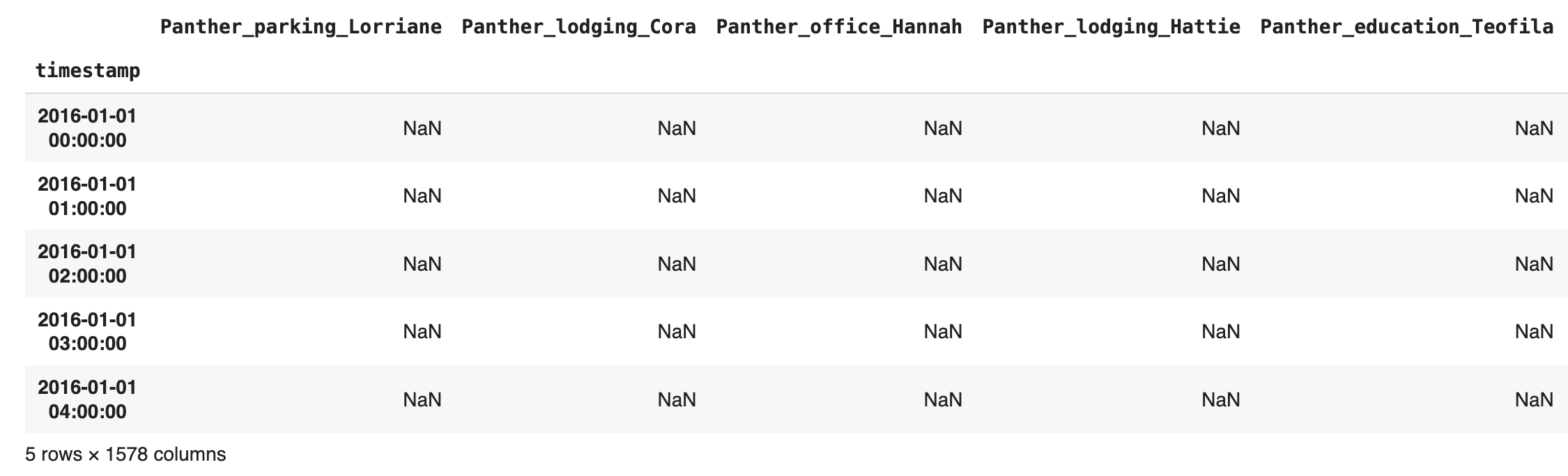
Every building in the dataset is represented by a column, while each row represents a hourly timestamp. Each building (column) has an anonymyzed unique identifier that follows the structure: Animal name (unique per location) + Simplified Usage + Human-like name (unique per building). E.g: Raven_education_Nina.
In this example we will look at a building located in Washington DC: Rat_education_Alfonso (Rat is the prefix used in BDG2 for Washington DC city buildings). Let’s extract and plot the electricity consumption data from the building:
# Create a new dataframe with only the data the selected building

building_df = meters_df['Rat_education_Alfonso']
building_df = building_df.rename('consumption')

# Plot the consumption timeseries with plotly

fig = go.Figure()
fig.add_trace(go.Scatter(x=building_df.index, y=building_df, name='consumption', line=dict(color='#007BFF')))
fig.show()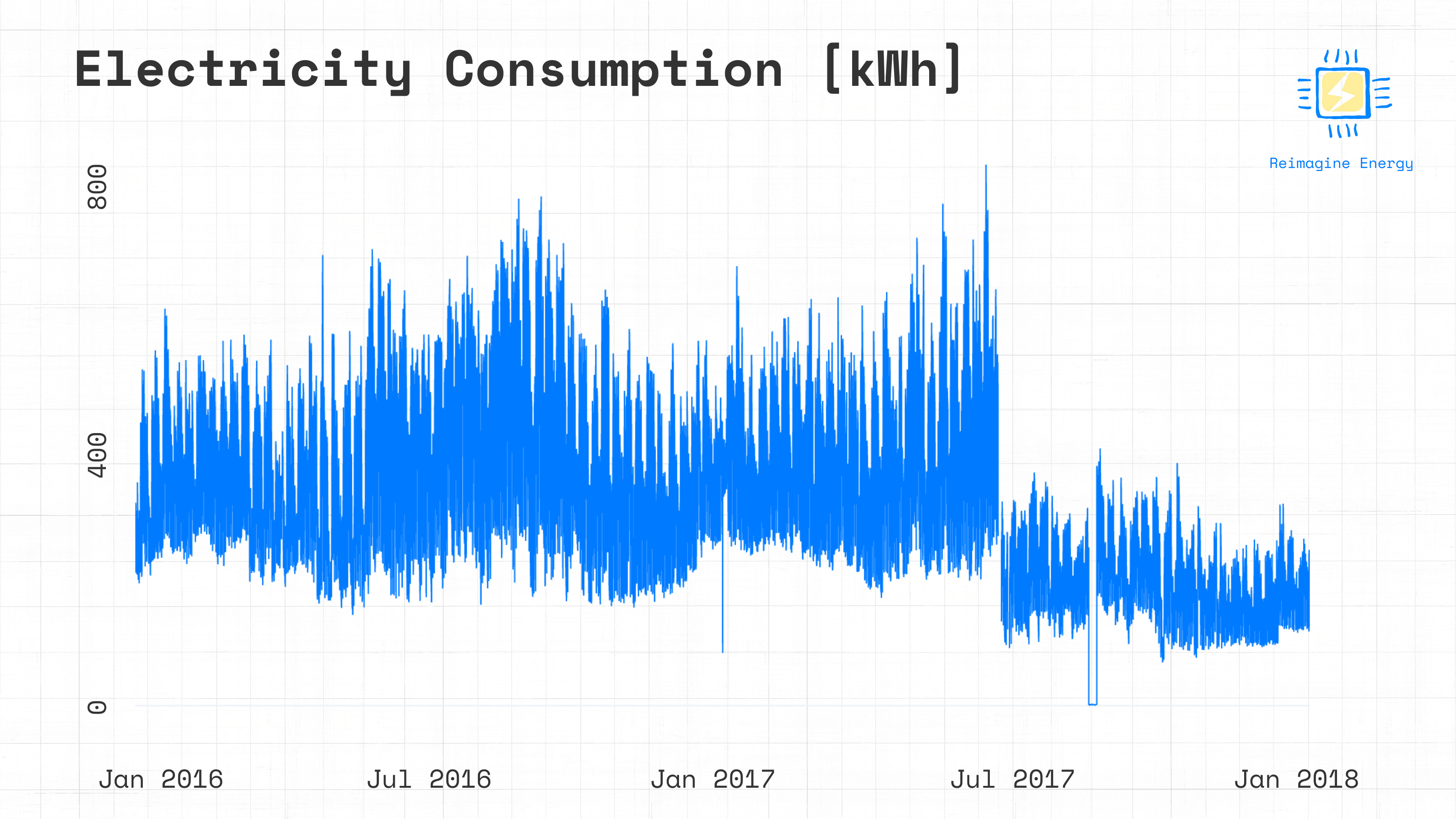
A closer look at the graph will show that some days of data are missing between June 20th and June 28th 2017, followed by a reduction in consumption. This is a typical indication of an energy efficiency measure installation period. We can then define the week between June 20th and June 28th as the installation period for the project we’re looking to verify. At a glance, it also looks like there are no major variations in consumption in the historical data before June 20th, so we can define the baseline period as the period between January 2016 and June 20th 2017, and the reporting data as the period between June 28th 2017 and December 2017.
# Define baseline, installation, and reporting period dates

installation_start = pd.to_datetime('2017-06-21')
installation_end = pd.to_datetime('2017-06-28')

baseline_start = building_df.index[0]
baseline_end = installation_start

reporting_start = installation_end
reporting_end = building_df.index[-1]
We’ll use these dates later to define the baseline and reporting period dataframes, which will serve as a basis for our analysis.
Weather Data
In order to build a counterfactual model for savings estimation, we’ll need information about the variables that are affecting the energy consumption of the analysed building. The two most common groups of features used in this case are occupancy data and weather data. It’s very rare to be able to access detailed occupancy data for individual buildings, for this reason calendar features are often used as a proxy for occupancy. Weather data, on the other hand, can be accessed more easily. In this case, the weather dataset has been directly provided within the BDG2 repository. Let's start by inspecting the weather data.
# Import weather data
weather_df = pd.read_csv('data/weather/weather.csv')

# Set the timestamp column as index of the dataframe

weather_df.set_index('timestamp', inplace=True)
weather_df.index = pd.to_datetime(weather_df.index)
weather_df.head()
Output
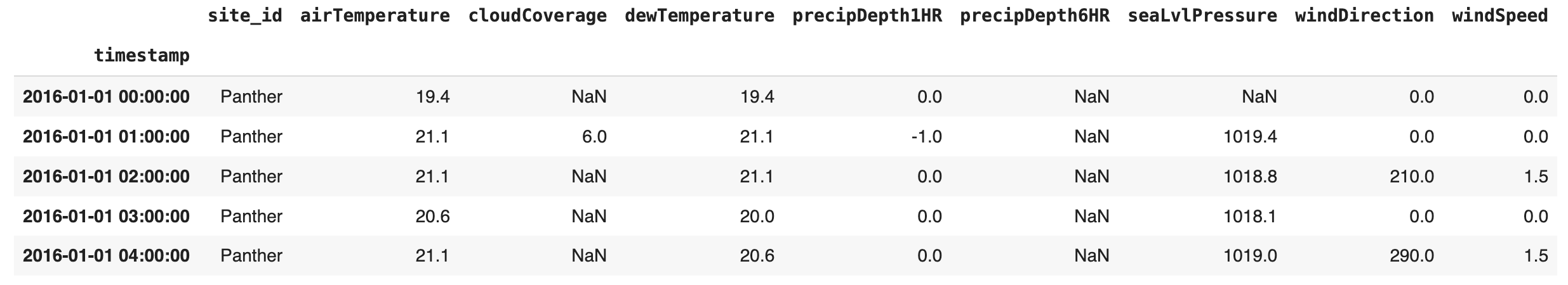
There’s eight different weather features, grouped by site location (indicated by the animal name). In our case, we are only interested in the location with id "Rat", that we know corresponds to a dataset of City Buildings from Washington DC2. Let’s perform a first quality check on the weather data, looking at the number of NaN values for each variable.
# select only columns where site id is 'Rat' and drop site id column
weather_df = weather_df[weather_df['site_id'] == 'Rat']
weather_df.drop('site_id', axis=1, inplace=True)

# Data quality check
# Print NaN values and the total length of the dataframe

print(weather_df.isna().sum())
print(f'Total DataFrame length: {len(weather_df)}')
Output
airTemperature        6
cloudCoverage      7497
dewTemperature        9
precipDepth1HR       49
precipDepth6HR    16846
seaLvlPressure      300
windDirection       290
windSpeed            11
dtype: int64
Total DataFrame length: 17539
A first analysis of the weather dataset shows that two variables (cloudCoverage and precipDepth6HR) are missing many datapoints, meaning they can't be used to build a model. Let’s exclude those variables and plot the rest to see if we can spot any other obvious issues in the data.
# Drop columns with missing data
weather_df.drop(['cloudCoverage', 'precipDepth6HR'], axis=1, inplace=True)

# Plot weather data
colors = ['#007BFF', "#9185FF", "#FFC107", "#FF5733", "#35AAD7", "#333333"]

fig = make_subplots(rows=2, cols=3, shared_xaxes=True, subplot_titles=weather_df.columns)

for i, col in enumerate(weather_df.columns):
    row = (i // 3) + 1   # Integer division determines the row
    col_idx = (i % 3) + 1  # Remainder determines the column

    fig.add_trace(
        go.Scatter(x=weather_df.index, y=weather_df[col], mode='lines', name=col,
                   line=dict(color=colors[i % len(colors)])),
        row=row, col=col_idx,
    )

fig.show()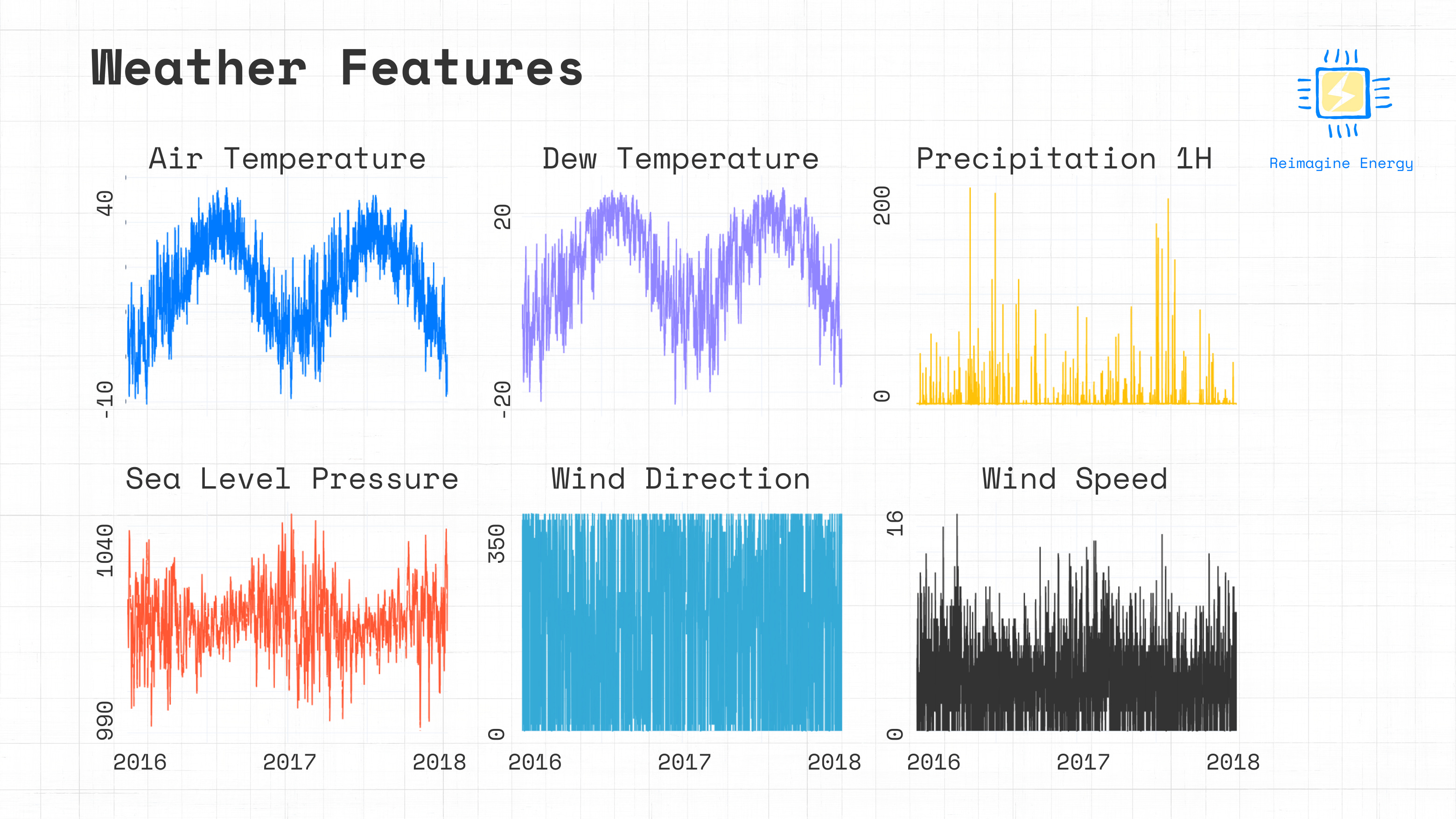
It looks like there’s no obvious outliers or problematic data from the plot, meaning that we can merge the consumption and weather datasets.
# Merge the dataframes using the index (timestamp)

df = building_df.to_frame().merge(weather_df, left_index=True, right_index=True)
Calendar Features
Another relevant feature which has an impact on the consumption of a building is occupancy. Accessing occupancy data from buildings is a challenging task, but we can replace that data with calendar features that can help the model understand the daily, weekly, and yearly trend of the energy consumption.
# Add calendar features
df["hour"] = df.index.hour
df["dayofweek"] = df.index.dayofweek
df["week"] = df.index.isocalendar().week.astype("int")
The final step before we can build our model is to split the full dataset between a baseline and a reporting dataset.
# Create baseline and reporting dataframes
baseline_df = df[(df.index >= baseline_start) & (df.index <= baseline_end)]

reporting_df = df[(df.index >= reporting_start) & (df.index <= reporting_end)]
Conclusion
That’s a wrap for this issue. With the baseline and reporting datasets ready, in the next article we’ll explore how to build a counterfactual energy model using gradient boosted trees. We will evaluate the importance of each feature in the model and then implement it to verify the actual savings achieved through the energy efficiency measures implemented in the building.
A comprehensive description of the Building Data Genome Project 2 dataset can be found on its dedicated Github page and associated scientific publication.
You can find a complete overview of the locations included in the dataset in this paper.