Case Study: Using AI to Verify Savings Across 9,000 Buildings
Ento's journey in evaluating energy crisis measures for 74 Danish municipalities
In September 2022, the Danish authorities decided to implement a range of energy conservation measures to counteract the effect of the energy crisis sparked by Ukraine’s invasion. These measures were designated for implementation across all municipalities as a response to the soaring energy prices.
Few months later, Ento was chosen by KL - Local Government Denmark, the central organization representing the interests of all Danish municipalities, to verify the impact of those energy conservation strategies. The experience we have at Ento with scalable analytics across extensive property portfolios, allowed us to thoroughly evaluate the impact of the energy crisis interventions and generate a public report.
Today’s issue of Reimagine Energy is part of a larger series on the role of AI in Measurement & Verification (M&V) practices. The previous two articles of the series featured a high-level introduction to the topic, and a deep-dive on the history and future of M&V. Today, I want to get more hands-on with a case study which will illustrate the verification process of energy efficiency savings within a substantial building portfolio. To my knowledge, there exists no other report in academic or industry literature covering in detail the methodology and results of such a large M&V project, so I believe that this post will be of value in unveiling the intricacies involved in such projects.
Project overview
Before getting into the methodological details, I’ll quickly introduce some practical information about the project. The main energy crisis measures that we were tasked to verify were the following:
Indoor temperature setpoint adjustment to 19 degrees Celsius for energy efficiency
Discontinuation of non-essential outdoor aesthetic lighting
Shortening of the heating season and reduction of heating and ventilation operational hours
Comprehensive energy conservation training for building occupants
Decreasing the delay before motion-activated lights turn off, in the absence of detected movement
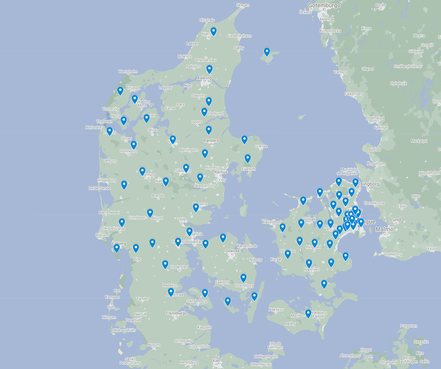
The study encompassed 74 out of the 98 Danish municipalities, with initial data being provided for about 14.000 buildings. The primary focus of the analysis was on electrical consumption data, which was sourced from the Danish electricity data hub. District heating savings were also analyzed, but but only for one municipality, due to data integration challenges. Individual municipalities often have several different district heating suppliers, requiring custom data integration efforts to access the consumption data.
For the project, we decided to align our methodology with the International Performance Measurement and Verification Protocol (IPMVP), a comprehensive standard outlined in detail in the previous newsletter issue. Among the different options provided for evaluating savings with this protocol, Option C (Whole Facility) was chosen. Option C provides a holistic approach to evaluating energy savings by comparing the actual energy consumption of a whole building after the implementation of an energy efficiency project, to what would have been consumed had the project not been implemented.
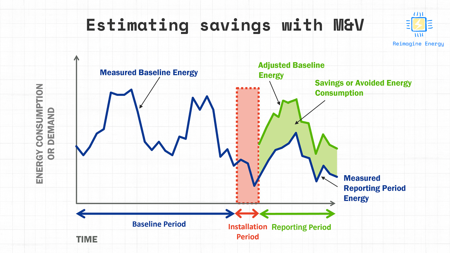
The approach involves establishing a baseline energy consumption level before the implementation of the measures and then measuring the actual energy consumption after the implementation. The difference between the two values is used to determine the energy savings achieved. A more detailed explanation of this process can be found in the first article of our series on M&V.
Option C determines the total savings of all implemented energy saving measures in a building, and is only applicable in projects where savings are expected to have a substantial impact, making them distinguishable from energy variations unrelated to the applied measures.
Methodology
The first step in the analysis was to integrate the metering data from the data portal and create “sites” on the Ento platform, corresponding to real buildings. This step was carried out with Ento’s advanced site allocation tool and proved necessary to aggregate data from several different electricity meters that might belong to a single building. Once the data was integrated and allocated to sites, the following steps were followed for each site:
The metering data was divided into:
Baseline period (before September 1st 2022)
Installation period (from September 1st to September 30th, 2022)
Reporting period (from October 1st 2022 to February 28th 2023)
A baseline (counterfactual) model was trained on data from the baseline period
The model error (CV(RMSE)) was calculated on holdout sets of the training data
If model error was higher than 30%, the model was retrained using only one year of training data (August 2021 to August 2022)
If the error was still greater than 30%, the site was deemed not fit for automated M&V and excluded from the analysis
Using the defined baseline model, the adjusted baseline energy consumption for the period October 2022 - February 2023 was calculated
The energy savings were calculated as the difference between the adjusted baseline energy consumption and the measured reporting period energy consumption
The cost and CO2 savings were calculated by multiplying the energy consumption by the relevant coefficients
The aggregated uncertainty range at 95% confidence level was estimated for the calculated savings
Once the calculations were run for each individual site, the savings and uncertainty of all sites were aggregated at municipality level.
The steps outlined are just a broad overview of the methodology used, and there’s multiple details that could be explored further. Here I will focus on three key aspects: the baseline model, the error metric, and the uncertainty of the results.
Baseline consumption model
We decided to use a gradient boosting decision tree to build the consumption model, due to its speed, accuracy, and reliability. The following explanatory features were included in the model:
Calendar features (day of the week, week of the year)
Periods corresponding to Covid-19 stay-at-home measures
Danish bank holidays
Outdoor temperature
Solar irradiation
Wind speed and direction
Precipitation intensity
Although the electricity consumption data integrated from Energinet had hourly or sub-hourly frequency, we decided to run the model on daily aggregated values. We decided to use a daily model since several studies have shown that when using hourly models there is a tendency to underestimate the uncertainty of the results because of the autocorrelation of residuals. An additional motivation was that, for this specific project, there was no interest in knowing the specific hour at which savings happened, but only the aggregated value of the savings month by month.
Error metric - CV(RMSE)
The metric chosen to evaluate the validity of the results was the Coefficient of Variation of the Root Mean Square Error (CV(RMSE)). This metric is calculated by dividing the Root Mean Square Error (RMSE) by the mean of the observed data. This normalization allows for the comparison of model accuracy across datasets with different scales or units. It is particularly useful in building energy modeling, where energy consumption values can vary greatly depending on the size, type, and usage of the building.
Where:
yi represents the actual observed values,
y^i represents the predicted values by the model,
yˉ is the mean of the actual observed values,
n is the number of observations in the dataset.
The CV(RMSE) is frequently used as an error metric to evaluate counterfactual models for M&V projects, being the reference metric mentioned both in the IPMVP and in the ASHRAE Guideline 14. The 30% threshold value used to exclude buildings from the analysis was arbitrarily set to include as many buildings as possible in the study, while keeping high accuracy of estimated savings results.
Savings uncertainty estimation
Quantifying modeling uncertainty of aggregated energy saving values is no trivial task. Practitioners commonly use two strategies: a formula that was introduced in the ASHRAE Guideline 14, and k-fold cross-validation (CV) uncertainty estimation. The IPMVP does not have yet a clearly defined formula to estimate aggregated savings uncertainty. For this study, we decided to use the ASHRAE formula to estimate the uncertainty of the savings.
Where ∆ E is the uncertainty in the aggregated savings, n is the number of observations in the baseline period, m is the number of observations in the reporting period, Epreˉ is the mean of the actual energy consumption in the baseline period, Epost is the estimated energy consumption in the reporting period, 1.26 is an empirical factor of approximation used to avoid the matrix algebra of the original equation of the aggregated uncertainties, t is the t-statistic value which can be found in statistics books for a certain % of confidence, and MSE is the mean squared error of the baseline regression model.1
Intuitively, the uncertainty increases if the model error is high, if there’s a low number of baseline period observations (and a high number of reporting period observations), and depending on the ratio between the total reporting period consumption and the average baseline period consumption.
Results
While the primary focus of this article was on the methodology rather than the results, it’s also interesting to look at what our study uncovered. We analyzed in total over 14.000 buildings, across 74 municipalities, although only about 9000 were suitable for our automated M&V analysis due incomplete data. The total estimated electricity savings over the 5 months reporting period amounted to 33.98 GWh, equal to approximately 12.5% of the total estimated consumption for that period. This translated into 4085 tons of CO2 and over 11 million euros saved! The estimated savings uncertainty, at a 95% confidence level, was approximately ±0.53%.
As part of this study, we created several visualizations to present our results in different and intuitive ways. I include here two of those that stood out for me.
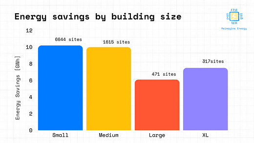
In the first one, we looked at which types of buildings were driving the most savings. The buildings were categorized based on their average monthly consumption during the reporting period:
Small from 0 to 5 MWh (6644 sites)
Medium from 5 to 15 MWh (1615 sites)
Large from 15 to 25 MWh (471 sites)
XL greater than 25 MWh (317 sites)
The largest buildings according to this classification saved together more than 7 GWh (an impressive average of 22 MWh per building). At the same time, and contrary to popular belief, smaller buildings were the highest contributors to overall savings, challenging the notion that energy efficiency efforts should only target larger buildings
.
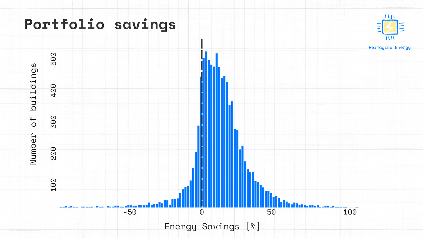
The second key insight, unveiled by the next graph, is the importance of evaluating savings across a portfolio rather than individually. Although there was variability within the savings of individual buildings, the implementation of multiple energy-saving measures across a large portfolio showed a positive general trend.
The hesitancy of major financing entities to engage in energy efficiency projects has historically been associated with the perception of limited scale and high uncertainty regarding the savings. Individual projects may seem too small to pique the interest of large investors, and the variability in potential savings can be off-putting, given the difficulty in predicting accurate returns.
However, the savings histogram illustrates a key concept: while individual buildings may exhibit variability in energy savings, a diversified approach across a sizable portfolio of buildings tends to yield a positive aggregate effect, counterbalancing the performance fluctuations within single buildings. Implementing standardized projects across a large portfolio can then help with risk mitigation, while also increasing the overall scale of the investment, making it more attractive to large financial institutions. While the energy conservation measures considered in our case study were mostly zero-cost, such an analysis would extend also to other types of actions that require an investment, such as LED installations, HVAC system retrofits etc.
Final remarks
Working on this project was a rewarding experience, not just for the results achieved and the technical challenge, but also for the satisfaction that came with contributing to a study of significant national impact in Denmark. The validation of the municipalities’ efforts in reducing energy consumption, will hopefully contribute to broader conversations about the impact of energy efficiency strategies across the country.
The success of the project was largely attributable to the sophisticated architecture and robust platform that we built at Ento. Once we had delineated the methodological parameters of the analysis, the process of integrating and assigning data to specific sites was remarkably smooth. Moreover, the seamless integration with our cloud computing infrastructure enabled the efficient execution of the machine learning calculations involved. Interestingly, the project inspired us to overhaul the savings verification module on our platform entirely. We introduced a tool compliant with IPMVP standards, designed to facilitate quick and easy verification of energy savings across an organization’s building portfolio with just a few clicks.
That’s a wrap for today, hopefully you enjoyed the article and I’ll see you in the next issue!


