Code Tutorial: Simulating Rooftop Solar Energy with Python

A Beginner’s Guide Using pvlib

In this tutorial, we will learn how to simulate the energy production of a rooftop photovoltaic energy system using the Python library pvlib. This tutorial is the first in a series that will focus on analyzing rooftop solar systems and matching its energy output with the building’s electricity consumption, with the goal of determining the optimal system capacity and its cost-effectiveness.

We will be working with the same building we analyzed in the counterfactual energy models tutorial. This building is located in Washington DC and has energy consumption data for the years 2016 and 2017.

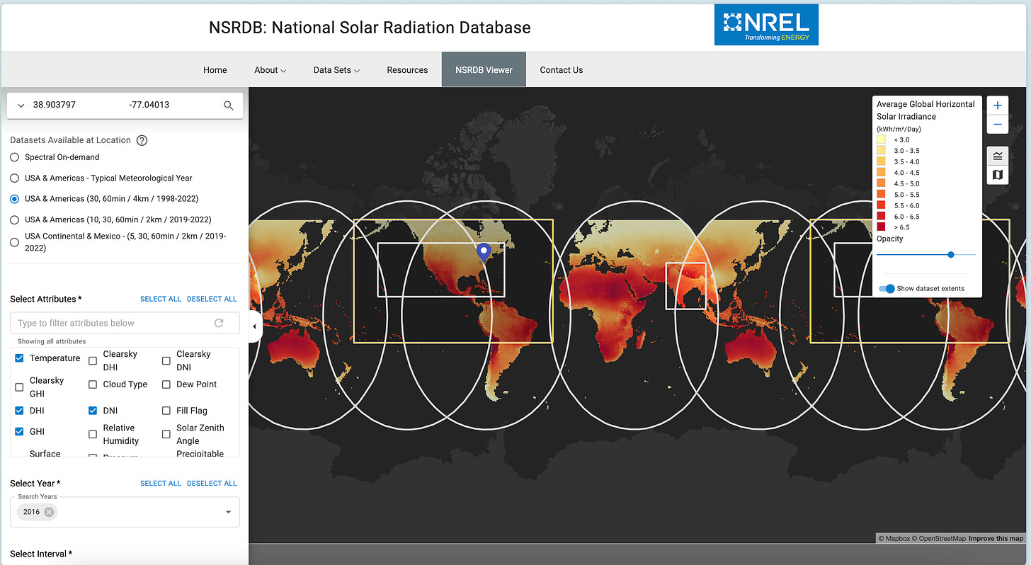
First, let’s download weather data for Washington DC for the year 2016. There are multiple platforms and APIs that let us access historical weather data. In this case, I used the National Solar Radiation Database from the NREL. Here’s how to do it:

1. Go to the NREL database link.

2. Enter “Washington, District of Columbia” as the location.

3. Select the “USA & Americas (30, 60min / 4km / 1998-2022)” dataset

4. Choose the following variables to include in the dataset: GHI, DNI, DHI, Temperature, Relative Humidity, Wind Speed, and Wind Direction.

5. Remember to mark the “Convert UTC to local time” checkbox.

For those who want to replicate this specific tutorial without downloading the data from the platform, here’s the XLSX file I used.

washington_dc_weather_2016

429KB ∙ XLSX file

Download

Download

Now that we have all the data we need, let’s import the necessary libraries for this tutorial. We will use the latest pvlib version, which is 0.11.0.

import math
import pandas as pd
import plotly.graph_objects as go

import pvlib
from pvlib.modelchain import ModelChain
from pvlib.pvsystem import PVSystem
from pvlib.location import Location

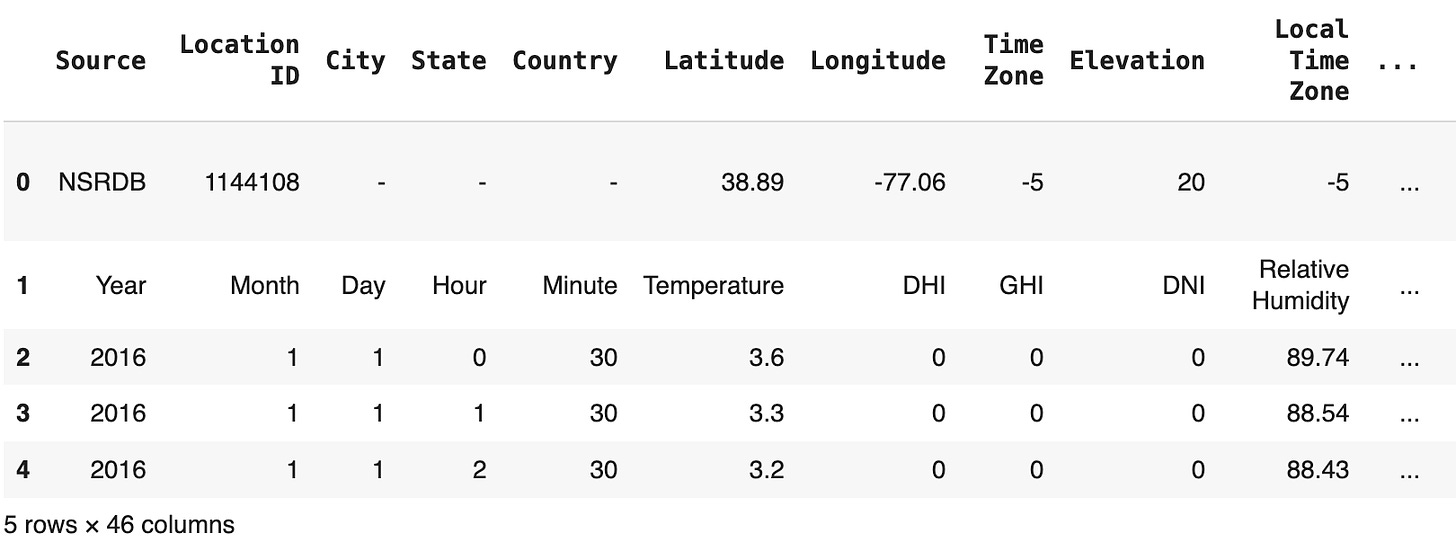
Let’s inspect the weather file we have downloaded.

weather_df = pd.read_excel('data/washington_dc_weather_2016.xlsx')
weather_df.head()

It looks like some data preprocessing is required to remove unnecessary rows and columns. We’ll also want to create a datetime index for our analysis.

#drop the first row and change the header
weather_df = weather_df.drop(0)
weather_df.columns = weather_df.iloc[0]
weather_df = weather_df.drop(1)

# create new datetime column using the columns year, month, day, hour, minute
weather_df['datetime'] = pd.to_datetime(weather_df[['Year', 'Month', 'Day', 'Hour', 'Minute']])
weather_df.set_index('datetime', inplace=True)
weather_df.index = pd.to_datetime(weather_df.index)

# resample to hourly
weather_df = weather_df.resample('H').mean()

# rename columns to use the pvlib nomenclature
weather_df = weather_df.rename(
            {
                "Temperature": "air_temp",
                "Wind Speed": "wind_speed",
                "Relative Humidity": "humidity",
                "Precipitable Water": "precipitable_water",
                "GHI": "ghi",
                "DNI": "dni",
                "DHI": "dhi",
            },
            axis=1,
        )

# convert values to float
weather_df['air_temp'] = weather_df['air_temp'].astype(float)
weather_df['wind_speed'] = weather_df['wind_speed'].astype(float)
weather_df['humidity'] = weather_df['humidity'].astype(float)
weather_df['precipitable_water'] = weather_df['precipitable_water'].astype(float)
weather_df['ghi'] = weather_df['ghi'].astype(float)
weather_df['dni'] = weather_df['dni'].astype(float)
weather_df['dhi'] = weather_df['dhi'].astype(float)

# select only relevant columns
weather_df = weather_df[['air_temp', 'wind_speed', 'humidity', 'precipitable_water', 'ghi', 'dni', 'dhi', ]]

# resample to hourly
weather_df = weather_df.resample('H').mean()
weather_df.head()

The weather dataframe looks much cleaner now. With the weather data ready, we can now define a PV system. We will use the Znshine 295 Wp panel model and an ABB 300W microinverter . While newer models can reach up to 400 Wp, this tutorial focuses on demonstrating the method, allowing the specific panel model and inverter to be easily changed later. For this tutorial, we will assume the system has a 35-degree tilt angle and the panels are oriented south (180 degrees).

# retrieve the inverter and panel specifications from the pvlib library

cec_modules = pvlib.pvsystem.retrieve_sam("cecmod")
sapm_inverters = pvlib.pvsystem.retrieve_sam("cecinverter")
module = cec_modules["Znshine_PV_Tech_ZXP6_72_295_P"]
inverter = sapm_inverters["ABB__MICRO_0_3_I_OUTD_US_208__208V_"]
temperature_model_parameters = pvlib.temperature.TEMPERATURE_MODEL_PARAMETERS[
    "sapm"
]["open_rack_glass_glass"]

# Create a Location and a PV System
location = Location(
    latitude=38.9072,
    longitude=-77.0369,
    name="Washington DC",
    altitude=0,
    tz='US/Eastern',
)

system = PVSystem(
        surface_tilt=35,
        surface_azimuth=180,
        module_parameters=module,
        inverter_parameters=inverter,
        temperature_model_parameters=temperature_model_parameters,
    )

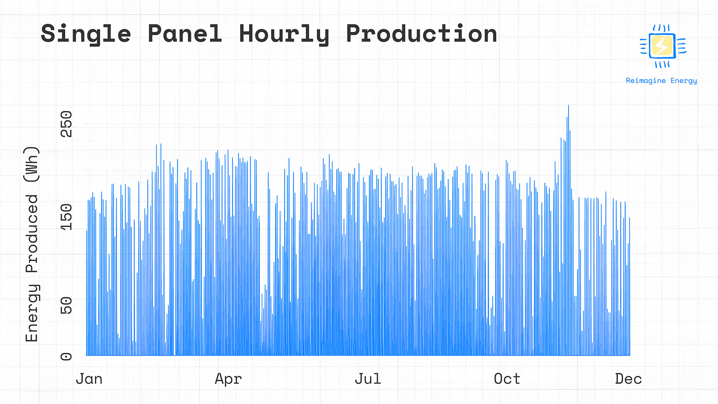
Now we can simulate the electricity generated by a single panel over one year at this location. The only parameter that we need to specify here, apart from the system characteristics and the location, is the angle of incidence (AOI) model. This is the loss model used to account for the reduction in solar irradiance due to the angle at which sunlight strikes the solar panels. In this case we opt for a physical model to calculate AOI losses based on the material properties of the panel’s surface.

# Create and run PV Model
mc = ModelChain(system, location, aoi_model="physical")
mc.run_model(weather=weather_df)
module_energy = mc.results.ac.fillna(0)

# Plot the estimated energy produced by a single panel

fig = go.Figure()
fig.add_trace(go.Scatter(x=module_energy.index, y=module_energy, mode='lines'))
fig.update_layout(yaxis_title='Energy Produced (kWh)')
fig.show()

The pattern suggests seasonal variations, with slightly higher hourly energy production in the warmer months and lower in the colder months, plus some outlier peaks in November.

Let’s now suppose we have an area of 400 m2 that we want to cover with solar panels. Assuming their inclination is 35 degrees, we can calculate how many panels will fit in this area.

# Define panel dimensions and peak power for Znshine_PV_Tech_ZXP6_72_295_P

panel_height = 1.95
panel_width = 0.99
panel_peak_power = 295
tilt_angle = 35
orientation = 180

# Calculate the area occupied by the PV panel on a flat roof
panel_area_flat_roof = (
        panel_height
        * panel_width
        * math.cos(tilt_angle * math.pi / 180)
    )

# calculate amount of panels that fit in a certain roof area
roof_area = 400
panel_count = math.floor(roof_area / panel_area_flat_roof)

# calculate the peak capacity of this system in kWp
system_peak_capacity = panel_count * panel_peak_power / 1000

print(f"Based on the specified system characteristics, {panel_count} panels can be installed on a {roof_area} m² flat roof. \nThis corresponds to a total system capacity of {system_peak_capacity} kWp.")

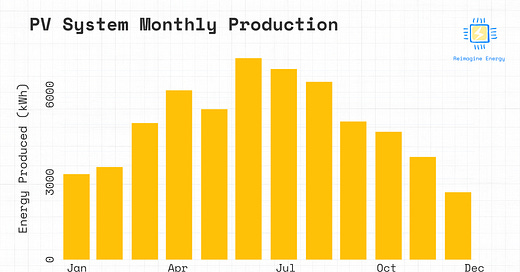
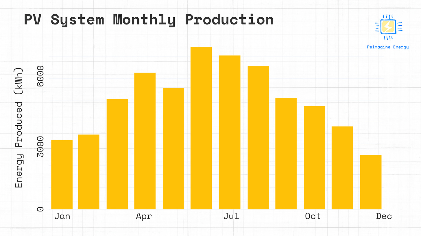
Finally, we can estimate the total annual production of this 74.34 kWp system. For this estimate, we are simplifying by assuming that the total system production will scale linearly with the number of panels. In reality, system-level effects such as shading from nearby objects, soiling, and thermal effects due to panel arrangement can impact performance. However, for the sake of this tutorial, this simplification is acceptable. We will also divide the result by 1000 to convert the results from Wh to kWh.

# Calculate the monthly production of the entire PV installation 
system_production = panel_count * module_energy / 1000
monthly_production = system_production.resample('M').sum()

# Plot monthly production
fig = go.Figure()
fig.add_trace(go.Bar(x=monthly_production.index, y=monthly_production))
fig.update_layout(yaxis_title='Energy Produced (kWh)')
fig.show()

It’s quite interesting to see how, despite the fact that the single panel’s hourly peak production is only slightly different across the seasons, the total monthly production varies significantly (more than doubling from January to June). This implies that the increased system production during summer is not strictly due to higher production at peak times, but rather to having more hours of daylight each day, leading to longer periods of energy production. The effect of having more hours of daylight is more significant than differences in peak panel production between winter and summer.

Conclusion

In this tutorial, we demonstrated how to simulate the annual energy production of a photovoltaic system using just a few lines of Python code and a weather dataset. In the upcoming episodes of this series, we will explore how to align the estimated production with a building’s electricity consumption timeseries to determine the optimal system capacity. Additionally, we will compare the pvlib methodology with other methods used to simulate the operation of a photovoltaic system.