Is solar estimation now as easy as an API call?

Comparing Google’s Solar API with traditional physics-based modeling

Can you estimate a building’s solar potential with just one API call? Google’s new Solar API claims to do just that. But how accurate is it compared to traditional methods?

I previously wrote a tutorial on estimating a building’s solar potential using pvlib, a physics-based simulation tool. With Google’s recent release of their Solar API, I couldn’t resist comparing the two methods. Could Google’s API really make solar estimation as easy as an API call?

In this comparison, I set out to evaluate two main factors:

1. Area of the Roof Suitable for Solar Panels: The total surface area where panels can be installed.

2. Production Potential per Panel: How much energy each panel can produce, considering factors like orientation, tilt, and local weather conditions.

Setting the Stage: Selecting a Rooftop in Washington DC

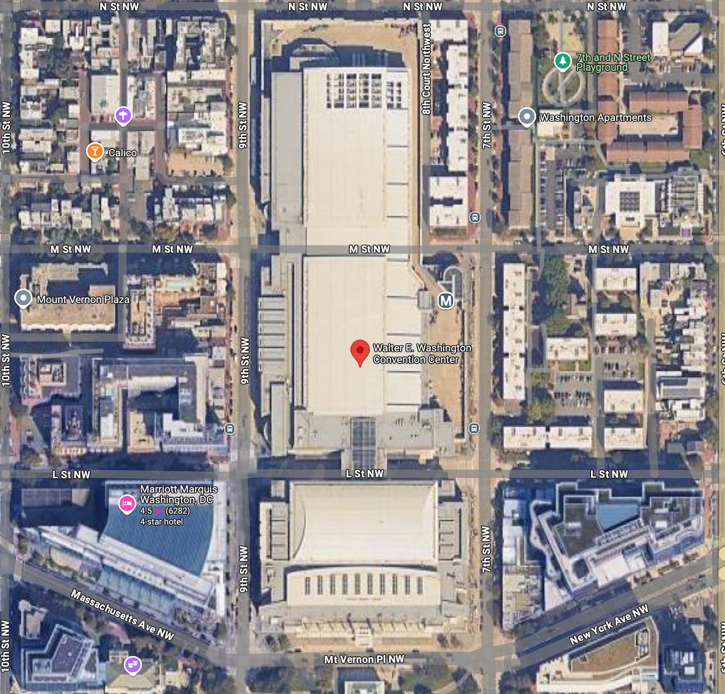
For this comparison, I chose a large rooftop in Washington DC. In the previous tutorials we’ve been analysing the consumption from a large facility located in Washington DC. We don’t have the building’s exact location, so I arbitrarily selected a large site in Washington DC with the help of Google Maps. The selected site is the Walter E. Washington Convention Center.

First Variable: Roof Area Suitable for Solar Panels

Manual Calculation Using Google Maps

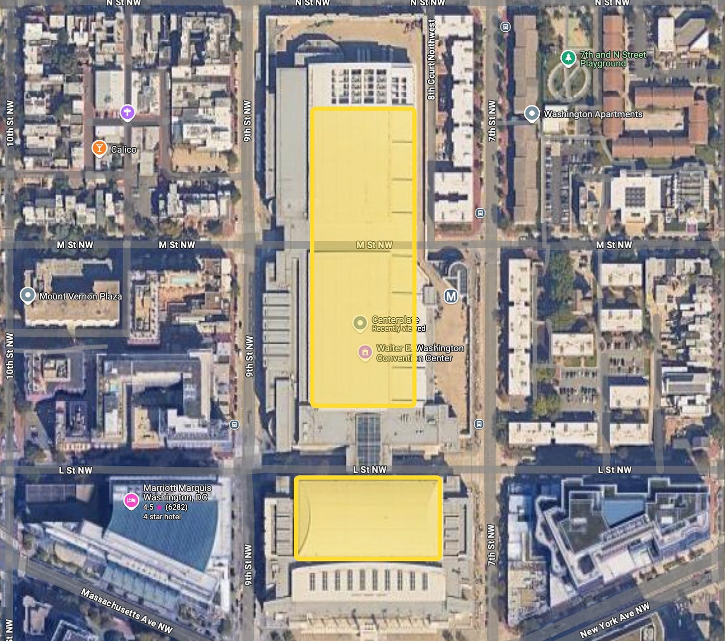
By inspecting the site on Maps, I identified two main roof segments suitable for solar panels:

I then used the Google Maps measure distance tool to estimate the total area available for the panels.

# Area available for solar panels according to manual calculations

area_segment_1 = 6000
area_segment_2 = 16500
total_roof_area = area_segment_1 + area_segment_2
print(f'Total area available for solar panels with manual calculation: {total_roof_area} m²')

Output

Automatic Calculation Using Google Solar

Next, I used Google’s Solar API to see what area it detects as suitable.

# Google Solar API call

import requests

api_key = 'your_api_key'
lat = 38.9052
lng = -77.0230
solar_request = requests.get(
    f"https://solar.googleapis.com/v1/buildingInsights:findClosest?location.latitude={lat}&location.longitude={lng}&requiredQuality=HIGH&key={api_key}"
)
solar_info = solar_request.json()

# Area available for solar panels according to the API
print(f'Area available for solar panels according to the Google Solar API: {round(solar_info["solarPotential"]["maxArrayAreaMeters2"])} m²')

# Percentage difference between the two calculations
percentage_difference = ((solar_info['solarPotential']['maxArrayAreaMeters2'] - total_roof_area) / total_roof_area) * 100
print(f'Percentage difference between the two calculations: {round(percentage_difference, 2)}%')

Output

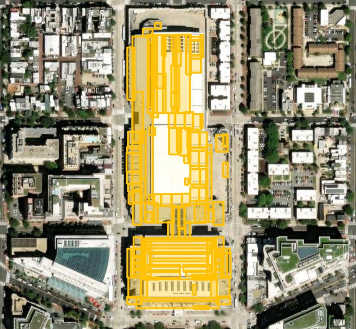
The area detected by the API is almost 30% larger than our manual measurement. To understand better where the difference is from, let’s plot the bounding boxes of the roof segments detected by Google Solar.

# Plot bounding boxes for detected roof segments

import plotly.graph_objects as go

# Prepare data
bounding_boxes = [roof_segment['boundingBox'] for roof_segment in solar_info['solarPotential']['roofSegmentStats']]
data = []
for bbox in bounding_boxes:
    sw = bbox['sw']
    ne = bbox['ne']
    data.append({
        'lat': [sw['latitude'], sw['latitude'], ne['latitude'], ne['latitude'], sw['latitude']],
        'lon': [sw['longitude'], ne['longitude'], ne['longitude'], sw['longitude'], sw['longitude']]
    })
    
# Create the figure
fig = go.Figure()


for d in data:
    fig.add_trace(go.Scattermapbox(
        lat=d['lat'],
        lon=d['lon'],
        mode='lines',
        fill='toself',
        line=dict(width=2, color='blue'),
        fillcolor='rgba(0, 0, 255, 0.3)',
        name='Roof Segment'
    ))

# Set up the map layout
fig.update_layout(
    mapbox=dict(
        style='white-bg',
        layers=[
            dict(
                sourcetype='raster',
                source=[
                    'https://server.arcgisonline.com/ArcGIS/rest/services/World_Imagery/MapServer/tile/{z}/{y}/{x}'
                ],
                below="traces"
            )
        ],
        center=dict(lat=lat, lon=lng),
        zoom=17
    ),
    margin={"r":0,"t":0,"l":0,"b":0}
)

# Display the map
fig.show()

Output

The API’s detected areas don’t align perfectly with the actual roof segments. Some of the identified areas are actually occupied by technical installations, and a large portion of the roof is not being detected.

Second Variable: Number of Panels Fit on the Roof

Google Solar’s estimate

The Solar API provides the maximum number of panels that can be installed.

# Maximum number of panels according to Google Solar
max_panels_api = solar_info['solarPotential']['maxArrayPanelsCount']
panel_capacity = solar_info['solarPotential']['panelCapacityWatts']
panel_height = solar_info['solarPotential']['panelHeightMeters']
panel_width = solar_info['solarPotential']['panelWidthMeters']

print(f"Maximum number of panels (Google Solar API): {max_panels_api}")
print(f"Panel Capacity: {panel_capacity} Wp")
print(f"Panel Dimensions: {panel_height} m x {panel_width} m")

Output

Google estimates we can fit a maximum of 14,648 400 Wp panels on this roof.

Pvlib’s estimate

To make a fair comparison, I selected a similar 400 Wp SunPower panel model. In order to access it, I had to download the latest CEC modules and inverter database, available on the NREL Github.

import pvlib

# Get panel and inverter models

cec_modules = pvlib.pvsystem.retrieve_sam(
    path="data/CEC Modules.csv"
)
cec_inverters = pvlib.pvsystem.retrieve_sam(
    path="data/CEC Inverters.csv"
)

# Choose a 400W panel and inverter
module = cec_modules["SunPower_SPR_MAX3_400"]
module_width = 1.69
module_length = 1.05
inverter = cec_inverters["SunPower__SPR_A400_H_AC__240V_"]

# Calculate how many panels fit in the area identified initially
module_area = module_width * module_length
max_panels_manual = round(total_roof_area/module_area)
print(f"Maximum number of panels (manual estimation): {max_panels_manual}")

Output

Comparing Annual Energy Production

Finally, let’s compare the annual energy production estimated with these two methods.

To run the pvlib calculations, we’ll suppose that the weather_df, temperature_model_parameters, and location variables are already available from the previous tutorial. Let’s simulate the production of one 400 Wp module in Washington DC with pvlib. The Google Solar API assumes that solar panels are installed flush with the roof surface. This means that the inclination of the panels is the same as the pitch of the roof segment they are mounted on. I selected a 5 degrees tilt for the pvlib system, since from the satellite image it doesn’t look like the roof has a significant inclination.

from pvlib.pvsystem import PVSystem
from pvlib.modelchain import ModelChain

# Define PV system characteristics
system = PVSystem(
        surface_tilt=5,
        surface_azimuth=180,
        module_parameters=module,
        inverter_parameters=inverter,
        temperature_model_parameters=temperature_model_parameters,
    )

# Create and run PV Model
mc = ModelChain(system, location, aoi_model="physical")
mc.run_model(weather=weather_df)
module_energy = mc.results.ac.fillna(0)

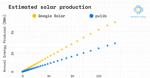
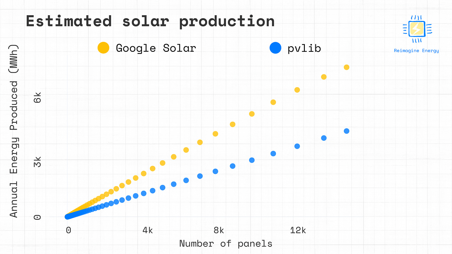
The Google Solar API returns a list of configurations with different numbers of panels. Let’s compare the expected annual solar production as estimated with pvlib and by the API.

import pandas as pd

# Get the list of configurations proposed by the Solar API
panel_configs = solar_info['solarPotential']['solarPanelConfigs']

# Select configurations evenly
step = len(panel_configs) // 50
selected_configs = panel_configs[::step]
# Add the last configuration if it's not already included
if panel_configs[-1] not in selected_configs:
    selected_configs.append(panel_configs[-1])

# Extract panel counts and yearly energy production for each configuration
panel_counts_selected = [config['panelsCount'] for config in selected_configs]
yearly_energy_selected = [config['yearlyEnergyDcKwh'] for config in selected_configs]
inverter_efficiency = 0.95  # Assume 95% efficiency

# Create a DataFrame
data = {
    'panels_count': panel_counts_selected,
    'solar_api_estimated_production': [energy * inverter_efficiency for energy in yearly_energy_selected],
    'pvlib_estimated_production': [(panel_count * module_energy / 1000).sum() for panel_count in panel_counts_selected]
}
df_configs = pd.DataFrame(data)

# Compare the production estimated with the two methods for different configurations

fig = go.Figure()

fig.add_trace(go.Scatter(
    x=df_configs['panels_count'],
    y=df_configs['solar_api_estimated_production'],
    mode='markers',
    marker=dict(
        size=10,
        color='#ffc107',
        opacity=0.8
    ),
    name='Google Solar'
))

fig.add_trace(go.Scatter(
    x=df_configs['panels_count'],
    y=df_configs['pvlib_estimated_production'],
    mode='markers',
    marker=dict(
        size=10,
        color='#007bff',
        opacity=0.8
    ),
    name='PVLIB'
))

fig.update_layout(
    xaxis_title='Number of Panels',
    yaxis_title='Annual Energy Produced',
    showlegend=True
)

fig.show()

Output

The Google Solar estimation provides a considerably higher estimated production, compared to the physical modelling method. Let’s quantify the difference for the configuration with the maximum number of panels.

# Calculate the percentage difference between Solar API and PVLIB estimates for the configuration with the highest number of panels

max_panels_count = df_configs['panels_count'].max()

# Fetch the solar production estimated by the Google Solar API for the maximum panels count
solar_api_production = df_configs[df_configs['panels_count'] == max_panels_count]['solar_api_estimated_production'].values[0]

# Fetch the solar production estimated by PVLIB for the same maximum panels count
pvlib_production = df_configs[df_configs['panels_count'] == max_panels_count]['pvlib_estimated_production'].values[0]

# Calculate the percentage difference between Google Solar API and PVLIB estimates
percentage_difference = ((solar_api_production - pvlib_production) / pvlib_production) * 100

# Print the results
print(f"Total annual energy production estimated by Google Solar API: {solar_api_production:.2f} kWh")
print(f"Total annual energy production estimated by PVLIB: {pvlib_production:.2f} kWh")
print(f"Percentage difference between Google Solar API and PVLIB estimates at max panel count: {round(percentage_difference, 1)}%")

Output

Although this is a preliminary analysis, it definitely raises some questions about the accuracy and reliability of Google’s Solar API for detailed solar potential assessments. Some potential reasons for the discrepancy might be:

• Weather Data Differences: We used 2016 weather data in the pvlib calculations, while Google Solar might be using a Typical Meteorogical Year or other data.

• Panel Model Variations: While we tried to match the panel specifications, there might be differences affecting efficiency.

• Assumptions in Shading and Losses: Google’s API might be making different assumptions about shading from nearby buildings, system losses, or other factors that influence production.

While the area detection difference might be due to computer vision errors—which is understandable in automated processes—the significant discrepancy in energy produced is concerning. It’s hard to justify a 74% difference based solely on data inputs or minor model variations.

Conclusion

Our comparison reveals significant differences between the two methods:

• Roof Area Detection: The area detected by Google is almost 30% higher than our manual estimation.

• Production Estimates: Google’s estimated annual production for the largest PV system configuration is is 77% higher than pvlib’s.

These findings suggest that while Google’s Solar API offers a convenient way to estimate solar potential, it might not provide accurate results for detailed assessments. Relying solely on the API could lead to overestimations and impact investment decisions.

What’s Next?

Is this discrepancy an isolated case? To find out, in the next tutorial I’ll test more buildings in different locations. I’m also interested in investigating whether Google Solar considers shading in its estimations, and have a look at the financial analyses provided by the API.

Want to help?

Try using the Google Solar API on a building you’re interested in and compare the results with a physics-based model like pvlib. Share your findings with me—I’d be happy to include your analyses in the next issue of the newsletter!