

Can we power a building entirely with solar energy?
Can we power a building entirely with solar energy?
Let’s find out using Python

Solar power is on the rise globally, driven by falling installation costs and higher efficiencies. But what does it take to power an entire facility only with solar?
In this tutorial, we will analyze the interaction between a building's energy consumption and a rooftop photovoltaic (PV) system using Python. This is the second tutorial in our series focusing on rooftop solar systems and their integration with building energy consumption data to determine optimal system sizing and cost-effectiveness. The first tutorial can be found here.
We will continue working with the same facility we analyzed in the counterfactual energy models tutorial, located in Washington, D.C.
Loading the Consumption Data
First, let’s load the building’s electricity consumption data and calculate the monthly totals. The details of the following data loading process are available in the counterfactual energy models tutorial.
import pandas as pd

# Load consumption data

meters_df = pd.read_csv('data/electricity_cleaned.csv')
meters_df.set_index('timestamp', inplace=True)
meters_df.index = pd.to_datetime(meters_df.index)
building_df = meters_df['Rat_education_Alfonso'].rename('consumption')

# Let's have a quick look at the monthly consumption data

monthly_consumption = building_df.resample('M').sum()
monthly_consumption.head()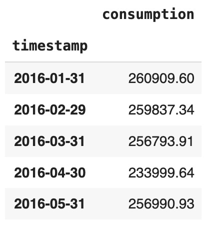
The monthly consumption for this building is around 260 MWh per month, which is very high. We’re likely looking at a large manufacturing facility or a group of buildings sharing one electricity meter.
Estimating the Required PV System Size
Next, we'll estimate the size of a PV system needed to meet the building's consumption using a simple engineering calculation.
From our last tutorial, we have the monthly production of a PV system in this location, and the system’s peak capacity. We can calculate the average kWh produced per kWp installed capacity for each month of the year. We’re assuming that the monthly production and system capacity variables are available from the previous tutorial.
# Calculate kWh produced per kWp of installed capacity each month
kwh_per_kwp = round(monthly_production / system_peak_capacity)
kwh_per_kwp = kwh_per_kwp.rename('monthly_kwh_per_kwp')
kwh_per_kwp.head()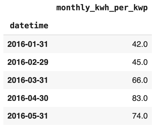
By comparing kwh_per_kwp with the building’s monthly consumption, we can estimate the required PV system size for each month.
# Calculate required PV system size for each month

monthly_data = pd.concat([monthly_consumption, kwh_per_kwp], axis=1)
monthly_data['required_size'] = round(monthly_data['consumption'] / monthly_data['monthly_kwh_per_kwp'])
monthly_data.head(12)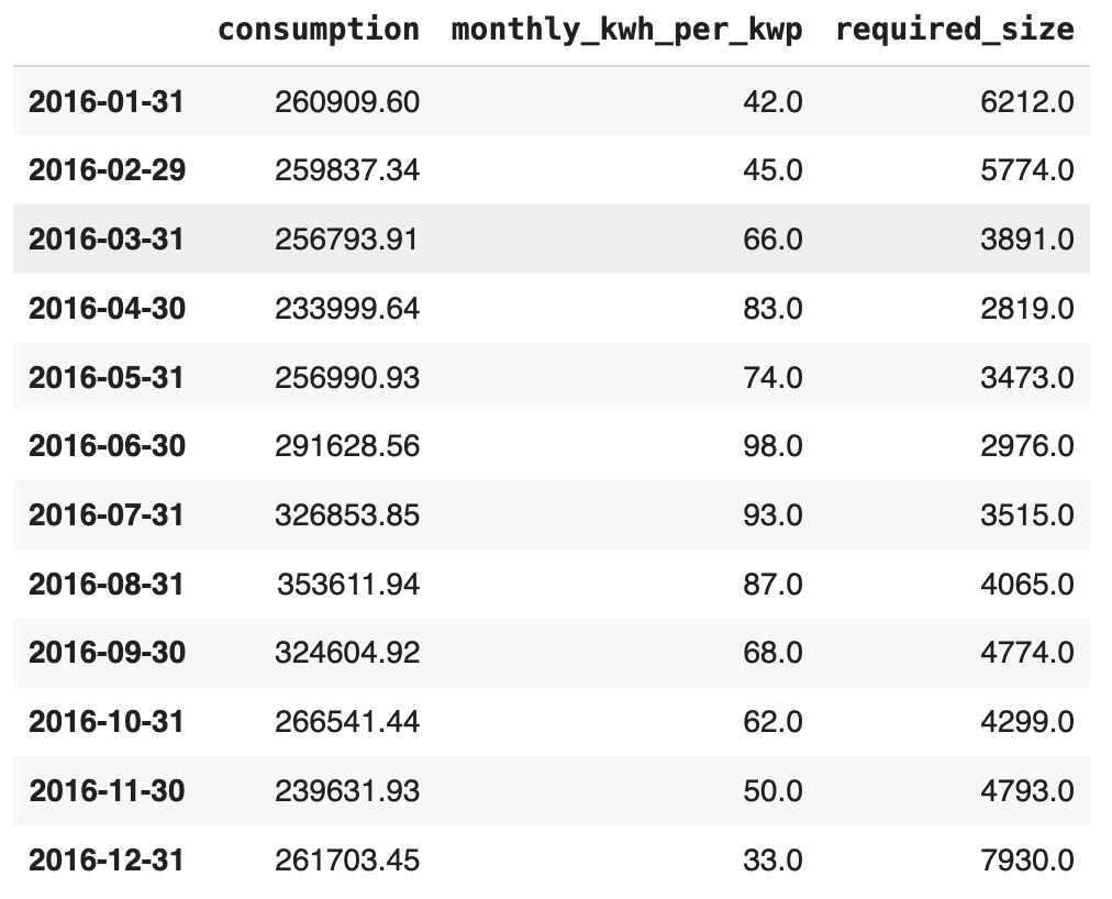
The table above shows the PV system size needed each month to match the building’s consumption. Since we’re using monthly data, this is a rough estimate with limitations. Even if monthly production matches consumption, they might not align in time.
To begin with, let’s base the system size on the average required capacity across the year. Note that since these calculations are done on monthly data, this is just a rough estimation based on a flawed reasoning. Production and consumption could happen at completely different times. But we need some criteria to decide on a size, and this is a good place to start.
# Specifications for the panel we chose in the previous tutorial
panel_height = 1.95
panel_width = 0.99
panel_peak_power = 295
tilt_angle = 35
orientation = 180

# Calculate the area occupied by the PV panel on a flat roof
panel_area_flat_roof = (
        panel_height
        * panel_width
        * math.cos(tilt_angle * math.pi / 180)
    )

# Calculate panel count and required roof area
system_capacity_kwp = monthly_data['required_size'].mean()
panel_count = system_capacity_kwp * 1000 / panel_peak_power
roof_area = panel_count * panel_area_flat_roof

print(f"According to the energy consumption matching method, {int(panel_count)} panels are required, covering {roof_area:.1f} m² of roof area.")
This is a very large system, that would typically be found in large-scale commercial or industrial installations.
Analyzing Consumption and Production Interaction
Now, let’s calculate the monthly production of this PV system. We’ll use the module energy data calculated in the previous tutorial, equivalent to the hourly energy output of a panel.
We'll calculate the building's grid consumption and export, after taking into account the PV production.
# Calculate system production, assuming module_energy is available from previous calculations
system_production = panel_count * module_energy / 1000  # Convert Wh to kWh

# Combine consumption and production data
data = pd.concat([building_df, system_production], axis=1).dropna()
data.columns = ['consumption', 'pv_production']

# Calculate grid import and injection
data['grid_flow'] = data['pv_production'] - data['consumption']
data['grid_import'] = data['grid_flow'].clip(upper=0)
data['grid_injection'] = data['grid_flow'].clip(lower=0)grid_importrepresents energy imported from the grid (when consumption exceeds production)grid_injectionrepresents excess energy sent back to the grid (when production exceeds consumption)
Results Visualisation
Let’s visualize the daily energy consumption before and after considering PV production.
# Daily data
daily_data = data.resample('D').sum()

# Plot daily consumption with and without PV
fig = go.Figure()
fig.add_trace(go.Scatter(x=daily_data.index, y=daily_data.consumption, line=dict(color='#7ac53c')))
fig.add_trace(go.Scatter(x=daily_data.index, y=-daily_data.grid_import, line=dict(color='#007BFF')))

fig.add_trace(
        go.Scatter(
            x=daily_data.index,
            y=daily_data.consumption,
            mode="lines",
            showlegend=False,
            line=dict(color="rgba(135, 197, 95, 0.2)", width=0),
            fill="tonexty",
            fillcolor="rgba(135, 197, 95, 0.2)",
        )
    )

fig.show()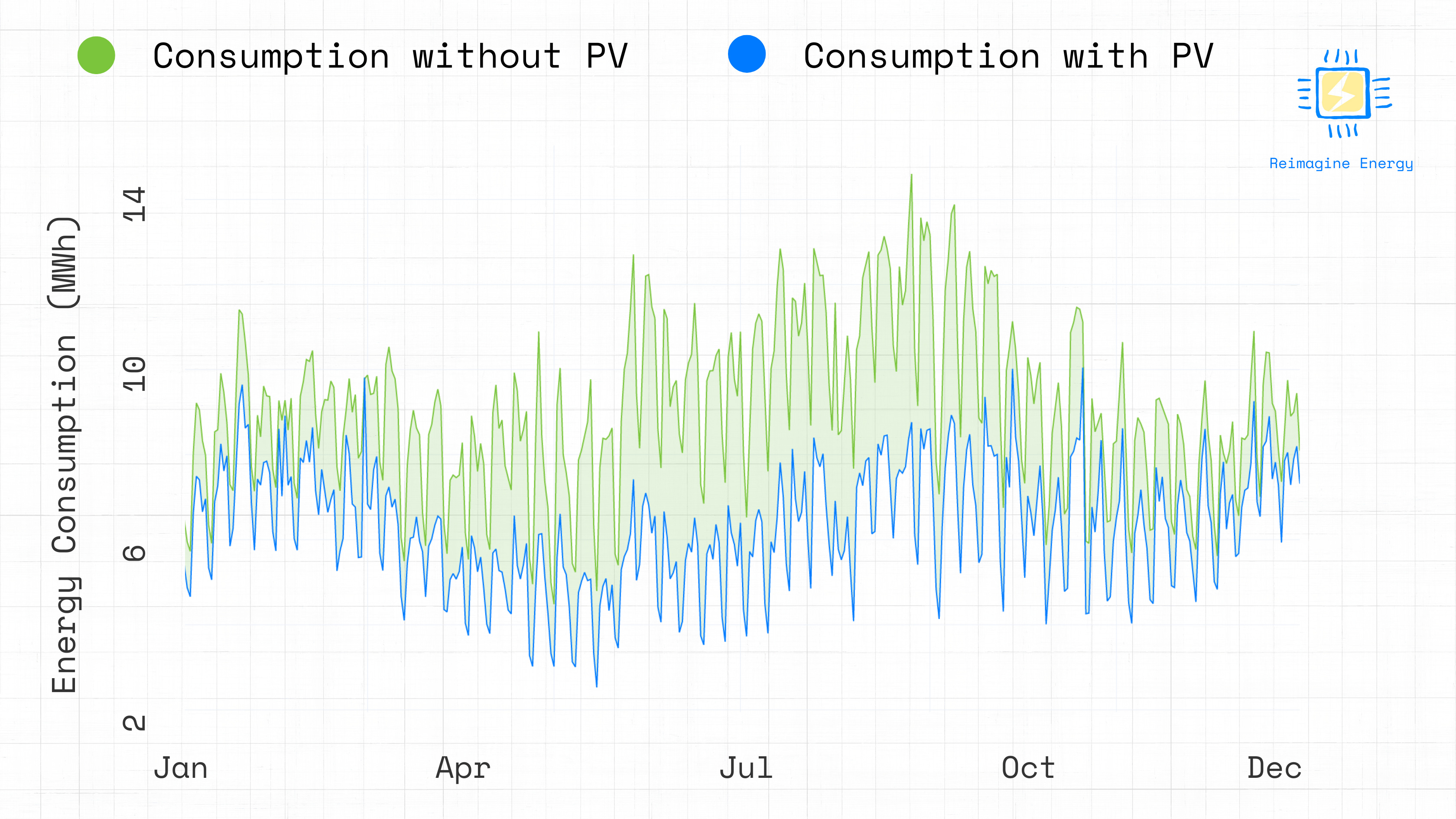
This line chart compares the daily energy consumed from the grid before and after installing the PV system.
Let’s also look at the monthly energy flows to get a comprehensive view.
# Plot monthly breakdown of energy consumed, produced, and exported

fig_monthly_breakdown = go.Figure()

fig_monthly_breakdown.add_trace(
    go.Bar(
        x=data.resample("M").sum().index,
        y=-data["grid_import"].resample("M").sum(),
        name="Grid Consumption",
        marker_color="#007BFF",
    )
)

fig_monthly_breakdown.add_trace(
    go.Bar(
        x=data.resample("M").sum().index,
        y=data["pv_production"].resample("M").sum(),
        name="Solar Production",
        marker_color="#ffc107",
    )
)

fig_monthly_breakdown.add_trace(
    go.Bar(
        x=data.resample("M").sum().index,
        y=data["grid_injection"].resample("M").sum(),
        name="Excess",
        marker_color="#9185ff",
    )
)

fig_monthly_breakdown.update_layout(
    barmode="group",
    xaxis_title="Date",
    yaxis_title="kWh",
    template="plotly_white",
)

fig_monthly_breakdown.show()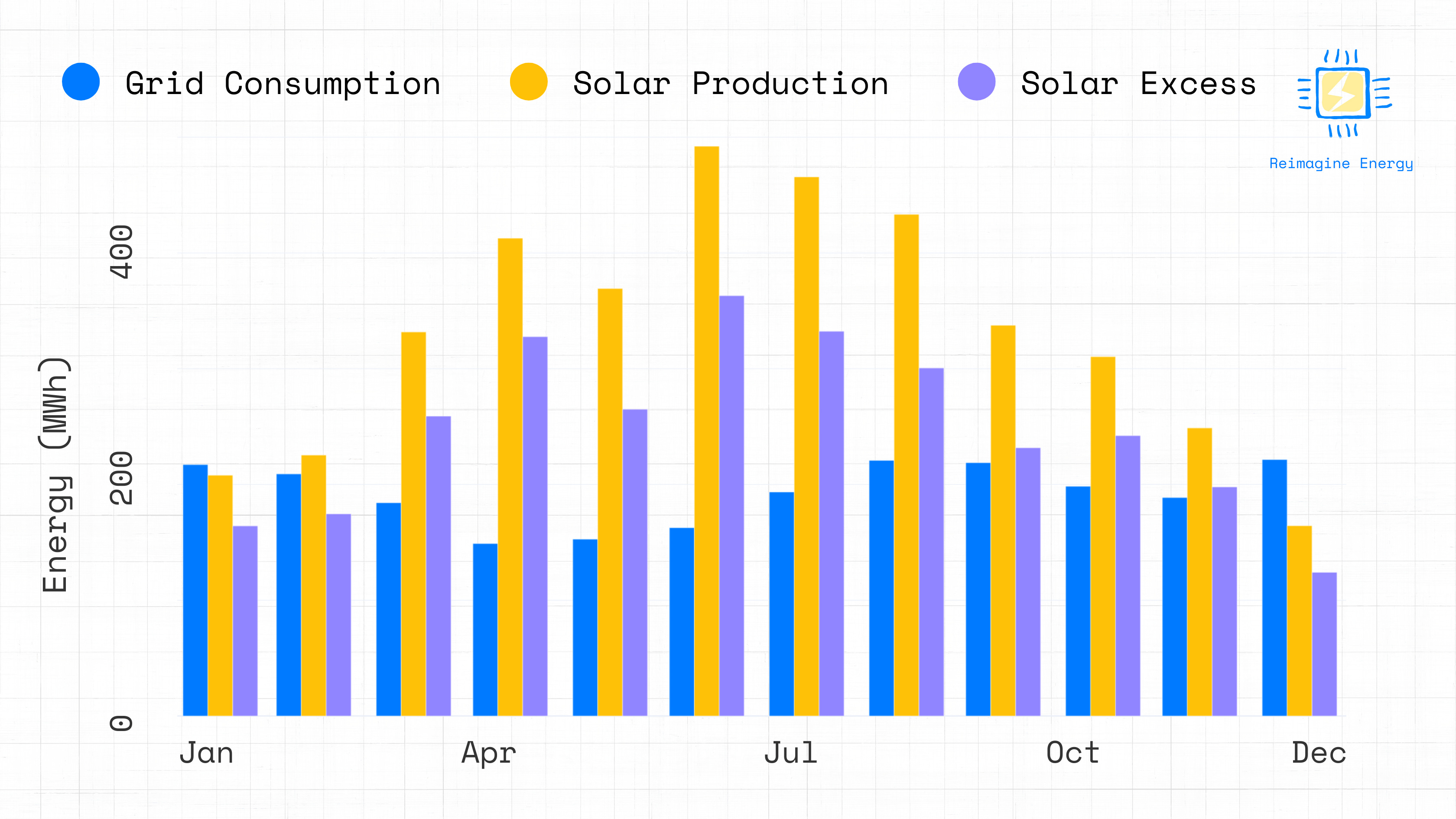
This grouped bar chart provides a clearer picture of how energy is consumed, produced, and exchanged with the grid each month.
Calculating Self-Consumption Metrics
Let’s compute some key metrics for the system.
# Calculate key metrics for the PV system

total_consumption = data['consumption'].sum()
total_production = data['pv_production'].sum()
grid_import = -data['grid_import'].sum()
grid_injection = data['grid_injection'].sum()
self_consumption = total_consumption - grid_import

self_consumption_percentage = (self_consumption / total_production) * 100
coverage_percentage = (self_consumption / total_consumption) * 100

print(f"Self-consumed energy: {self_consumption:.0f} kWh")
print(f"Percentage of total energy production that is self-consumed: {self_consumption_percentage:.1f}%")
print(f"Percentage of total energy consumption that is covered by PV self-consumption: {coverage_percentage:.1f}%")
Even with a large PV system, a substantial amount of electricity is still imported from the grid. This is because PV production doesn’t always match consumption times. Solar energy is generated during the day, but consumption is likely peaking at other times.
Estimating the Payback Time
Finally, let’s estimate how long it would take for such a system to pay for itself. We need to make some assumptions here:
• Electricity price: $0.10 per kWh
• Grid injection compensation: $0.05 per kWh
• System installation cost: $1,000 per kWp
# Financial calculations

electricity_price = 0.10
grid_compensation = 0.05
installation_cost_per_kwp = 1000

total_system_cost = system_capacity_kwp * installation_cost_per_kwp

annual_savings = self_consumption * electricity_price

annual_income = grid_injection * grid_compensation

total_annual_benefit = annual_savings + annual_income

payback_time = total_system_cost / total_annual_benefit

print(f"Total system cost: ${total_system_cost:,.0f}")
print(f"Annual electricity savings: ${annual_savings:,.0f}")
print(f"Annual income from excess energy: ${annual_income:,.0f}")
print(f"Estimated payback time: {payback_time:.1f} years")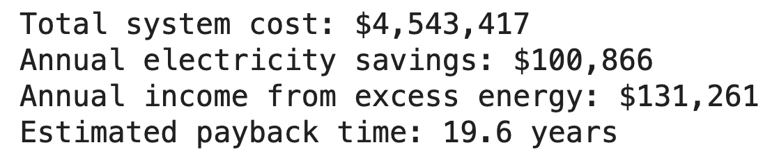
Conclusion
In this tutorial, we modeled the interaction between a building’s energy consumption and a rooftop PV system using Python. By estimating the required system size and analyzing performance metrics, we gained valuable insights into the potential benefits and challenges of integrating solar energy into building operations.
Despite installing a large PV system, we observed that a significant amount of energy is still imported from the grid due to the mismatch between production and consumption times. Furthermore, with current assumptions of installation costs, electricity price, and grid injection compensation, the payback time for this system is quite long. Energy storage solutions could enhance self-consumption rates and improve the system's cost-effectiveness.
To answer the initial question: powering this facility entirely with solar energy would require an extremely large system and massive energy storage. This may not be financially viable. Alternative approaches, like shifting consumption patterns or offsetting carbon emissions through Energy Attribute Certificates (EACs), might be better options to reach carbon neutrality.
For this tutorial, we mainly based our calculations on monthly consumption data available from the facility. In the next tutorials, we’ll explore a more complex sizing strategy that considers the building’s specific consumption patterns. This approach will help us identify optimal system capacities that guarantee lower payback times.